import matplotlib.pyplot as plt
import numpy as np
%matplotlib inline
from jupyterthemes import jtplot
plt.style.use('mike')
jtplot.style(context='talk', fscale=1, grid=False)

import cosmogrb

GRBs

This section describes how to handle the low level simulation of GRBs. AS the code currently is built for simulating GRBs as observed by Fermi-GBM, we will focus our attention there. As the code expands, I will update the docs.

Instantiate the GRB with its parameters

For this example, we will create a GRB that has its flux coming from a single pulse shape that is described by a cutoff power law evolving in time.

\[F_{h\nu}(t) = K(t) \left(\frac{\nu}{\nu_0(t)} \right)^{-\alpha} \cdot \exp\left(- \frac{\nu}{\nu_0(t)} \right)\]

grb = cosmogrb.gbm.GBMGRB_CPL(
    ra=312.0,
    dec=-62.0,
    z=1.0,
    peak_flux=5e-7,
    alpha=-0.66,
    ep=500.0,
    tau=2.0,
    trise=1.0,
    tdecay=1.0,
    duration=80.0,
    T0=0.1,
)

grb.info()

	0
name	SynthGRB
z	1
ra	312
dec	-62
duration	80
T0	0.1

	0
peak_flux	5.000000e-07
alpha	-6.600000e-01
trise	1.000000e+00
tdecay	1.000000e+00

	0

Examine the latent lightcurve

time = np.linspace(0, 20, 500)

grb.display_energy_integrated_light_curve(time, color="#A363DE");

---------------------------------------------------------------------------
IndexError                                Traceback (most recent call last)
<ipython-input-3-0737622692d6> in <module>
      1 time = np.linspace(0, 20, 500)
      2
----> 3 grb.display_energy_integrated_light_curve(time, color="#A363DE");
      4

~/coding/projects/cosmogrb/cosmogrb/grb/grb.py in display_energy_integrated_light_curve(self, time, ax, **kwargs)
    143         """
    144
--> 145         list(self._lightcurves.values())[0].display_energy_integrated_light_curve(
    146             time=time, ax=ax, **kwargs
    147         )

IndexError: list index out of range

energy = np.logspace(1, 3, 1000)

grb.display_energy_dependent_light_curve(time, energy, cmap='PRGn', lw=.25, alpha=.5)

Simulate the GRB

Now we can create all the light curves from the GRB. Since are not currently running a Dask server, we tell the GRB to process serially, i.e., computing each light curve one at a time.

grb.go(serial=True)

Save the GRB to an HDF5 file

As this is a time-consuming operation, we want to be able to save the GRB to disk. This is done by serializing all the light curves and information about the GRB into an HDF5 file.

grb.save('test_grb.h5')

Reload the GRB

What if want to reload the GRB? We need to create and instance of GRBSave from the file we just created. Notice all the information about the GRB is recovered.

grb_reload = cosmogrb.GRBSave.from_file('test_grb.h5')
grb_reload.info()

	0
name	SynthGRB
z	1
ra	312
dec	-62
duration	80
T0	0.1

	0
alpha	-6.600000e-01
peak_flux	5.000000e-07
tdecay	1.000000e+00
trise	1.000000e+00

The GRBSave contents

The stores all the information about the light curves and the instrument responses used to generate the data. Each light curve/ response pair can be accessed as keys of the GRBSave. Then one can easily, examine/plot/process the contents of each light curve.

for key in grb_reload.keys():

    lightcurve = grb_reload[key]['lightcurve']
    lightcurve.info()

	0
name	b0
instrument	GBM
tstart	-100
tstop	300
time adjustment	5.76246e+08
T0	0.1
n_counts	190656
n_counts_source	36
n_counts_background	190660

	0
angle	106.678116

	0
name	b1
instrument	GBM
tstart	-100
tstop	300
time adjustment	5.76219e+08
T0	0.1
n_counts	206738
n_counts_source	70
n_counts_background	206695

	0
angle	64.599896

	0
name	n0
instrument	GBM
tstart	-100
tstop	300
time adjustment	5.76253e+08
T0	0.1
n_counts	194080
n_counts_source	136
n_counts_background	194008

	0
angle	140.423466

	0
name	n1
instrument	GBM
tstart	-100
tstop	300
time adjustment	5.76276e+08
T0	0.1
n_counts	198594
n_counts_source	127
n_counts_background	198530

	0
angle	123.192564

	0
name	n2
instrument	GBM
tstart	-100
tstop	300
time adjustment	5.76203e+08
T0	0.1
n_counts	203221
n_counts_source	87
n_counts_background	203189

	0
angle	87.337115

	0
name	n3
instrument	GBM
tstart	-100
tstop	300
time adjustment	5.76206e+08
T0	0.1
n_counts	200535
n_counts_source	108
n_counts_background	200460

	0
angle	120.135933

	0
name	n4
instrument	GBM
tstart	-100
tstop	300
time adjustment	5.76229e+08
T0	0.1
n_counts	204014
n_counts_source	89
n_counts_background	203953

	0
angle	115.423396

	0
name	n5
instrument	GBM
tstart	-100
tstop	300
time adjustment	5.76212e+08
T0	0.1
n_counts	201485
n_counts_source	47
n_counts_background	201489

	0
angle	91.866668

	0
name	n6
instrument	GBM
tstart	-100
tstop	300
time adjustment	5.76284e+08
T0	0.1
n_counts	203790
n_counts_source	121
n_counts_background	203697

	0
angle	126.89814

	0
name	n7
instrument	GBM
tstart	-100
tstop	300
time adjustment	5.76264e+08
T0	0.1
n_counts	205853
n_counts_source	142
n_counts_background	205745

	0
angle	150.685788

	0
name	n8
instrument	GBM
tstart	-100
tstop	300
time adjustment	5.76264e+08
T0	0.1
n_counts	205156
n_counts_source	127
n_counts_background	205069

	0
angle	121.106339

	0
name	n9
instrument	GBM
tstart	-100
tstop	300
time adjustment	5.76252e+08
T0	0.1
n_counts	198283
n_counts_source	85
n_counts_background	198226

	0
angle	108.143856

	0
name	na
instrument	GBM
tstart	-100
tstop	300
time adjustment	5.76287e+08
T0	0.1
n_counts	198458
n_counts_source	582
n_counts_background	197918

	0
angle	57.909913

	0
name	nb
instrument	GBM
tstart	-100
tstop	300
time adjustment	5.76277e+08
T0	0.1
n_counts	206218
n_counts_source	206
n_counts_background	206091

	0
angle	77.225671

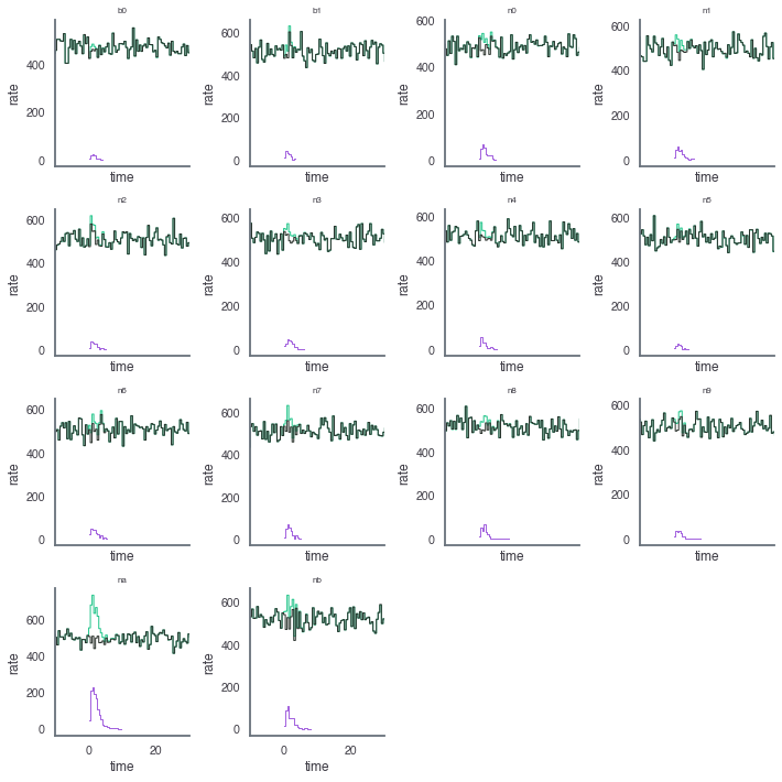
For example, let’s look at the total, source, and background data light curves generated.

fig, axes = plt.subplots(4,4,sharex=True,sharey=False,figsize=(10,10))
row=0
col = 0
for k,v  in grb_reload.items():
    ax = axes[row][col]

    lightcurve =v['lightcurve']

    lightcurve.display_lightcurve(dt=.5, ax=ax,lw=1,color='#25C68C')
    lightcurve.display_source(dt=.5,ax=ax,lw=1,color="#A363DE")
    lightcurve.display_background(dt=.5,ax=ax,lw=1, color="#2C342E")
    ax.set_xlim(-10, 30)
    ax.set_title(k,size=8)



    if col < 3:
        col+=1
    else:
        row+=1
        col=0

axes[3,2].set_visible(False)
axes[3,3].set_visible(False)
plt.tight_layout()

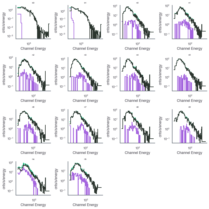
And we can look at the generated count spectra/

fig, axes = plt.subplots(4,4,sharex=False,sharey=False,figsize=(10,10))
row=0
col = 0

for k, v in grb_reload.items():
    ax = axes[row][col]

    lightcurve = v['lightcurve']

    lightcurve.display_count_spectrum(tmin=0, tmax=5, ax=ax,color='#25C68C')
    lightcurve.display_count_spectrum_source(tmin=0, tmax=5, ax=ax,color="#A363DE")
    lightcurve.display_count_spectrum_background(tmin=0, tmax=5, ax=ax, color="#2C342E")
    ax.set_title(k,size=8)

    if col < 3:
        col+=1
    else:
        row+=1
        col=0

axes[3,2].set_visible(False)
axes[3,3].set_visible(False)
plt.tight_layout()

Convert HDF5 to standard FITS files

In the case of GBM, we can convert the saved HDF5 files into TTE files for analysis in 3ML.

cosmogrb.grbsave_to_gbm_fits("test_grb.h5")
!ls SynthGRB_*

ls: SynthGRB_*: No such file or directory